
Monte Carlo integration is a technique for estimating the value of a definite integral using random sampling and then applying a deterministic method to estimate the integral.
For example, suppose we want to estimate the value of the integral f(x)dx from a to b. We can do this by randomly generating points in the interval [a,b] and then estimating the integral as the average value of f(x) at those points.
In other words, we are approximating the integral by a Riemann sum. The advantage of Monte Carlo integration is that it can be used to estimate integrals that are difficult or impossible to compute using traditional methods.
Monte Carlo integration
Monte Carlo integration takes a number of random points, which are used to calculate the area under a curve or on a definite integral equation.
As the number of random points increases, the more accurate our integration becomes. This basically implies that more random variates = more accuracy.
Example of Monte Carlo Integration
Approximate the integral \int_0^1x^2\ dx using the Monte Carlo method.
The code for the above steps is shown below.
#Set the number of values
n <- 10000
#Generate n random numbers on the interval [0,1]
x  <- runif(n,min=0,max=1)
#Evaluate the function at the random values of s
fx <- x^2
#Estimate the integral
integral <- mean(fx)*1 # Multiply by the base length 1-0
integral
[1] 0.3336095
This output may vary due to the degree of randomness set in our R program. In order to stop this variation, we need to use the command set. seed( )
Applying the set.seed() function in our Monte Carlo integration.
set.seed(123)

#Set the number of values
n <- 10000
#Generate n random numbers on the interval [0,1]
x  <- runif(n,min=0,max=1)
#Evaluate the function at the random values
fx <- x^2
#Estimate the integral
integral <- mean(fx)*1 # Multiply by the base length 1-0
integral
After executing the above R code, our output should be the same.
[1] 0.3297405
Example 2
Compute the exact value of the integral \int_0^64x^3 and use Monte Carlo integration to obtain a value of the estimate.
set.seed(123)

#Set the number of values
n <- 10000
#Generate n random numbers on the interval [0,6]
x  <- runif(n,min=0,max=6)
#Evaluate the function at the random values
fx <- 4*x^2
#Estimate the integral
integral <- mean(fx)*6 # Multiply by the base length 6-0
integral
[1] 284.8957
The exact value is 2888.
Example 3
Compute the integral \int_0^{\frac{\Pi}{3}}\sin\left(t\right)dt using monte carlo integration
set.seed(123)

#Set the number of values
n <- 10000
#Generate n random numbers on the interval
t  <- runif(n,min=0,max=pi/3)
#Evaluate the function at the random values
ft <- sin(t)
#Estimate the integral
integral <- mean(ft)*pi/3 # Multiply by the base length Pi-0
integral
[1] 0.49808
Example 4: Estimation of Pi using Monte Carlo Integration
# Monte Carlo estimation of Pi
set.seed(123)  # for reproducibility
n <- 10000     # number of random points

x <- runif(n)
y <- runif(n)

inside_circle <- sum(x^2 + y^2 <= 1)
pi_estimate <- 4 * inside_circle / n

cat("Estimated Pi:", pi_estimate, "\n")
Estimated Pi: 3.18
Example 4: Multidimensional Monte Carlo integration
Find the integral \int_0^{0.5}\int_0^{0.5}\int_0^{0.5}\frac{2}{3}\left(x_1+x_2+x_3\right)dx_1dx_2dx_3
To integrate a scalar function over a multidimensional rectangle, use the R function adaptIntegrate() from the library ‘cubature’
library(cubature)
f<- function(x){
  (2/3)*(x[1]+x[2]+x[3])
}
adaptIntegrate(f, lowerLimit = c(0,0,0), upperLimit = c(0.5,0.5,0.5))
> adaptIntegrate(f, lowerLimit = c(0,0,0), upperLimit = c(0.5,0.5,0.5))
$integral
[1] 0.0625

$error
[1] 1.387779e-17

$functionEvaluations
[1] 33

$returnCode
[1] 0
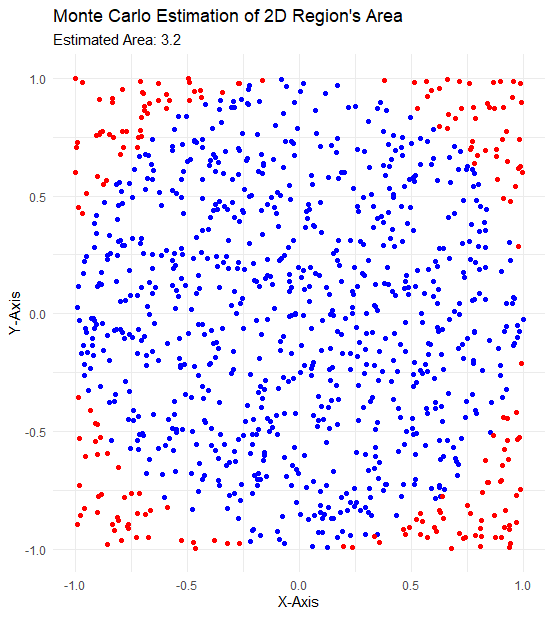
Example 5: Estimating a 2D region’s area
# Monte Carlo estimation of a 2D region's area
f <- function(x, y) x^2 + y^2 <= 1  # Function indicating the region

set.seed(123)
n <- 10000

x <- runif(n, -1, 1)
y <- runif(n, -1, 1)

inside_region <- sum(f(x, y))
area_estimate <- 4 * inside_region / n  # Multiplying by 4 to account for the entire square

cat("Estimated Area:", area_estimate, "\n")
Estimated Area: 3.1576
Let’s visualize the above 2D region area:
# Monte Carlo estimation and plot of a 2D region's area
library(ggplot2)

# Function indicating the region
f <- function(x, y) x^2 + y^2 <= 1

set.seed(123)
n <- 1000

x <- runif(n, -1, 1)
y <- runif(n, -1, 1)

inside_region <- f(x, y)
outside_region <- !inside_region

# Create a data frame for the points
df <- data.frame(x = x, y = y, inside = inside_region)

# Create the plot
ggplot(df, aes(x, y, color = inside)) +
  geom_point() +
  scale_color_manual(values = c("red", "blue"), guide = FALSE) +
  theme_minimal() +
  labs(
    title = "Monte Carlo Estimation of 2D Region's Area",
    subtitle = paste("Estimated Area:", sum(inside_region) / n * 4),
    x = "X-Axis",
    y = "Y-Axis"
  )
Additional Resources
Why are Monte Carlo Simulations used?