Distributions.
Distribution is the arrangement of values of a variable in order of magnitude. A distribution can be described as being symmetrical, skewed, uniform, random, or normal.
A distribution is said to be symmetrical if it is mirror-image symmetrical about the center. The most common type of symmetrical distribution is the normal distribution. A distribution is said to be skewed if one tail is longer than the other. The most common type of skewed distribution is the exponential distribution. A distribution is said to be uniform if all values are the same. A distribution is said to be random if it is not possible to predict the value of the variable.
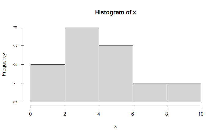
There are many ways to visualize a distribution in R. One way is to use a histogram. To create a histogram, you can use the hist() function. This function will take in a vector of values and will create a histogram with bars representing the frequency of each value in the vector.
You can also use the qplot() function to create a variety of different types of plots, including histograms, boxplots, and scatterplots. This function is part of the ggplot2 package, which must be installed and loaded before using qplot().
x <- c(1,3,5,6,3,4,2,9,8,5,3)
x
hist(x)
Normal Distribution
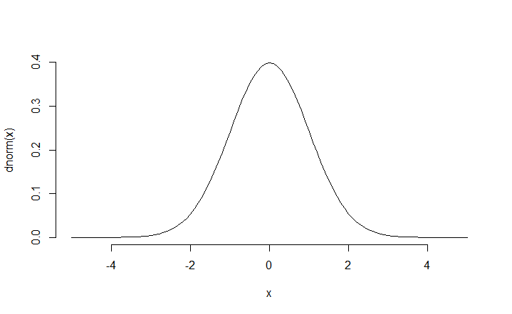
A normal distribution is a probability distribution that is symmetric about the mean, showing that data near the mean are more frequent in occurrence than data far from the mean. In a normal distribution, data are distributed evenly on either side of the mean, and the mean, median, and mode are all equal. The normal distribution is also known as the Gaussian distribution.
x = seq(-5, 5, 0.1)
plot(x = x, y = dnorm(x), type="l", bty="n")
There are 4 basic functions in R for calculating in the normal distribution.
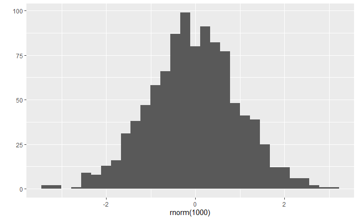
- rnorm\left(n,\ \mu,\ \sigma\right) generates n random values from a normal distribution with a mean \mu and a standard deviation sigma . If we omitted the parameters, R would default to \mu = 0 and \sigma = 1 .
qplot(rnorm(1000))
- pnorm\left(x,\ \mu,\ \sigma\right) is the cummulative distribution function (cdf) of the mormal distribution with mean \mu and standard deviation \sigma .
pnorm(10:14, 12, 0.8)
The above code basically means the probability of getting values 10, 11, 12, 13 and 14 with a mean of 12 and standard deviation of 0.8.
Output
[1] 0.006209665 0.105649774 0.500000000 0.894350226 0.993790335
- qnorm\left(p,\ \mu,\ \sigma\right) is the inverse of the cdf of the normal distribution with mean \mu and standard deviation \sigma . It returns the vlue such that pnorm\left(x,\ \mu,\ \sigma\right)=p .
qnorm(c(.25,.50,.75), 12, .8)
Output
[1] 11.46041 12.00000 12.53959
- dnorm\left(x,\ \mu,\ \sigma\right) is the probability density function of the normal distribution with mean \mu and standard deviation \sigma .
Example: Generate a normal distribution in R.
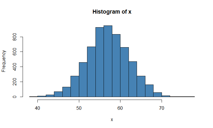
# To make sure that we get the same results for randomization.
set.seed(1)

#generate sample of 6000 observations that follows normal 4dist. with mean=57 and sd=5
X <- rnorm(6000,mean=57, sd=5)

#view first 6 observations in sample
head(x)

[1] 53.86773 57.91822 52.82186 64.97640 58.64754 52.89766
Let’s use a histogram to display the distribution of our random values x.
hist(x, col='steelblue')

Example 2
Simulate x-N(57,5) given that n=6000. Obtain the upper, lower limits and the number of outliers.
> #make this example reproducible
 set.seed(1)
#Generate sample of 6000 observations that follows normal dist. with mean=57 and sd=5
x <- rnorm(6000, mean=57,sd=5)
#View first 6 observations in sample
head(x)
[1] 53.86773 57.91822 52.82186 64.97640 58.64754 52.89766
#Find mean of sample
mean(x)
[1] 56.97696
 #Find standard deviation of sample
 sd(x)
[1] 5.094073
#Visualizing using a histogram
hist(x, col='steelblue')
#Plotting a boxplot to find upper and lower limit
bx <- boxplot(x)
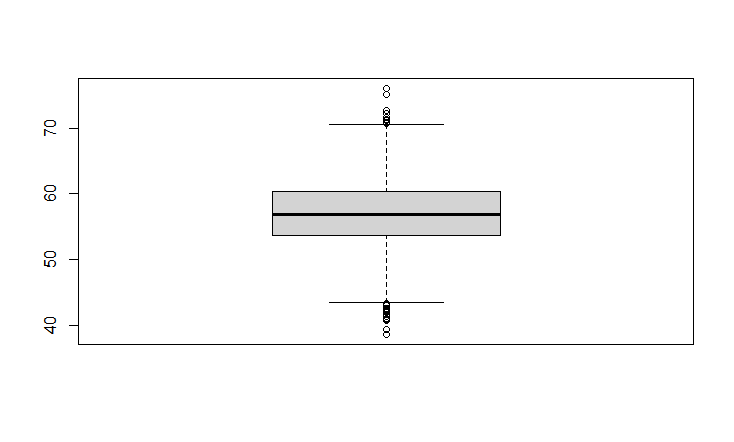
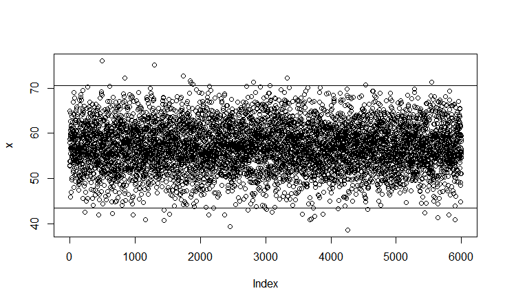
#Getting the limits of the boxplots
bx$stats
[1,] 43.52348 #Lower whisker
[2,] 53.65919 #Q1
[3,] 56.89197 #Q2 (median)
[4,] 60.44743 #Q3
[5,] 70.57166 #Upper whisker

#Plotting a scatter plot
plot(x)
#Using upper and lower limit
abline(h=43.52348)
abline(h=70.57166)
#Printing outlier values in the upper and lower limit
outliers <- boxplot.stats(x)$out
out
[1] 42.55540 41.95976 76.05138 42.30113 72.27871 42.01525 40.93406 75.19787 40.73390 43.02019
[11] 42.13871 72.76986 71.59614 71.20093 70.90694 41.88848 42.02449 39.30207 43.06993 71.31071
[21] 43.11204 42.57491 72.32262 42.09573 40.95972 40.98945 41.64378 42.13852 43.29674 38.64350
[31] 70.68485 43.18712 42.43587 71.30796 41.40441 41.99593 40.83695
#Finding the number of outliers exist
length(outliers)
[1] 37
#Outliers in the upper limit
for (i in outliers){
  if (i > 70.57166)
    print(i)
}
[1] 76.05138
[1] 72.27871
[1] 75.19787
[1] 72.76986
[1] 71.59614
[1] 71.20093
[1] 70.90694
[1] 71.31071
[1] 72.32262
[1] 70.68485
[1] 71.30796
#Outliers in the lower limit
for (j in outliers){
  if (j < 43.52348)
    print(j)
}
[1] 42.5554
[1] 41.95976
[1] 42.30113
[1] 42.01525
[1] 40.93406
[1] 40.7339
[1] 43.02019
[1] 42.13871
[1] 41.88848
[1] 42.02449
[1] 39.30207
[1] 43.06993
[1] 43.11204
[1] 42.57491
[1] 42.09573
[1] 40.95972
[1] 40.98945
[1] 41.64378
[1] 42.13852
[1] 43.29674
[1] 38.6435
[1] 43.18712
[1] 42.43587
[1] 41.40441
[1] 41.99593
[1] 40.83695