How to do Kaplan-Meier Survival Analysis in R

The Kaplan-Meier survival analysis, also known as the Kaplan-Meier estimator, is a non-parametric statistical method used to estimate the probability of an event (typically death, failure, or some other time-to-event outcome) occurring at a specific time in a dataset. It’s commonly used in medical research, clinical trials, and various other fields to analyze and visualize time-to-event data, where events may or may not have occurred for each individual in a study.

check out our FREE online statistics calculators

It considers both the time at which events occur and whether the events are censored. Censoring occurs when the exact event time is not observed for some individuals, but we know the event has not occurred by a certain time.

Here’s how Kaplan-Meier analysis works:

1. Data Preparation: You start with a dataset containing information about individuals, including their event times and whether or not the event of interest has occurred (often coded as 1 for the event and 0 for censored).
2. Calculating Survival Probabilities: The estimator calculates the probability of survival at different time points. It starts with an assumption that all individuals are alive (or event-free) at the beginning and calculates the probability of an event not occurring at each time point.
3. Product-Limit Estimator: Using the product-limit formula, the estimator computes the survival probability at each time point. Essentially, it multiplies the conditional probabilities of not experiencing an event up to that time point.
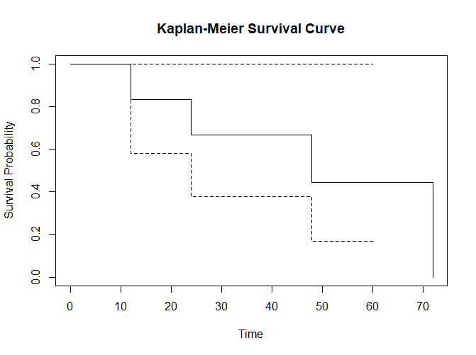
4. Plotting the Kaplan-Meier Curve: The results are typically visualized using a Kaplan-Meier survival curve, a step-like curve showing the estimated survival probability over time. The x-axis represents time, and the y-axis represents the estimated probability of survival.
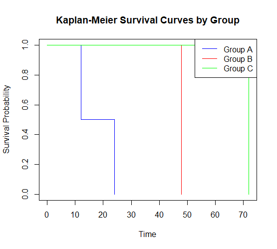
5. Comparing Groups: It can also compare survival curves between different groups or categories by stratifying the data and plotting separate Kaplan-Meier curves for each group. Statistical tests like the log-rank test can be used to assess the significance of differences between these curves.

Kaplan-Meier survival analysis is particularly useful when dealing with right-censored data, where not all individuals have reached the event of interest by the end of the study. It allows researchers to estimate and visualize the survival probabilities and to compare survival experiences between different groups. This method is essential for understanding the time-to-event data in clinical studies, epidemiology, and other fields where understanding the time until an event occurs is crucial.

Step 1: Install and Load Required Packages

You need to install and load the survival package if you haven’t already. You can install it using the following command:

install.packages("survival")

Once installed, load the package:

library(survival)

Step 2: Prepare Your Data

You’ll need a dataset with at least two variables: a time-to-event variable (usually called ‘time’) and a binary variable indicating whether an event occurred (usually called ‘status’ where 1 represents the event of interest, and 0 represents censoring). Your dataset can be in various formats, such as a data frame, but you should structure it like this:

# Example data frame
data <- data.frame(
  time = c(12, 24, 36, 48, 60, 72),
  status = c(1, 1, 0, 1, 0, 1)
)

Step 3: Perform Kaplan-Meier Analysis

You can use the survfit() function to estimate the Kaplan-Meier survival curve. Here’s how to do it:

# Fit Kaplan-Meier survival curve
fit <- survfit(Surv(time, status) ~ 1, data = data)

The Surv() function creates a survival object, and the formula Surv(time, status) ~ 1 specifies the time and status variables.

Step 4: Plot the Kaplan-Meier Curve

To visualize the Kaplan-Meier survival curve, you can use the plot() function:

# Plot the Kaplan-Meier curve
plot(fit, main = "Kaplan-Meier Survival Curve", xlab = "Time", ylab = "Survival Probability")

This will generate a simple Kaplan-Meier survival curve.

Step 5: Summarize Survival Probabilities

You can extract survival probabilities at specific time points and other summary statistics using the summary() function:

# Summary statistics
summary(fit, times = c(12, 24, 36, 48, 60, 72))

> summary(fit, times = c(12, 24, 36, 48, 60, 72))
Call: survfit(formula = Surv(time, status) ~ 1, data = data)

 time n.risk n.event survival std.err lower 95% CI upper 95% CI
   12      6       1    0.833   0.152        0.583            1
   24      5       1    0.667   0.192        0.379            1
   36      4       0    0.667   0.192        0.379            1
   48      3       1    0.444   0.222        0.167            1
   60      2       0    0.444   0.222        0.167            1
   72      1       1    0.000     NaN           NA           NA

This will provide you with survival probabilities at the specified time points.

Step 6: Compare Survival Curves

To compare survival curves between groups, you can use the survfit() function with a formula that includes a grouping variable. For example:

# Creating a grouped data frame
grouped_data <- data.frame(
  time = c(12, 24, 36, 48, 60, 72),
  status = c(1, 1, 0, 1, 0, 1),
  group = c("Group A", "Group A", "Group B", "Group B", "Group C", "Group C")
)

# Fit Kaplan-Meier survival curves by group
group_fit <- survfit(Surv(time, status) ~ group, data = grouped_data)

# Plot and compare survival curves
plot(group_fit, main = "Kaplan-Meier Survival Curves by Group", xlab = "Time", ylab = "Survival Probability", col = c("blue", "red", "green"))
legend("topright", legend = unique(grouped_data$group), col = c("blue", "red", "green"), lty = 1)

This will plot Kaplan-Meier curves for different groups and allow you to compare their survival probabilities.