How to Conduct Fisher’s Exact Test in R

Introduction

Fisher’s exact test is a non-parametric statistical test that helps us determine whether a significant association exists between two categorical variables in a contingency table. This test is particularly useful when dealing with small sample sizes or when the assumptions of the chi-squared test are not met.

Fisher’s exact test is often preferred over the chi-squared test when certain assumptions of the chi-squared test are not met. These assumptions include:

1. Sample Size: One of the primary assumptions of the chi-squared test is that it works well with large sample sizes. When the sample size is small, the chi-squared test may produce unreliable results, leading to inaccurate conclusions. Fisher’s exact test is better suited for situations with small sample sizes, making it a more appropriate choice.
2. Cell Frequencies: In a chi-squared test, it is assumed that each cell in the contingency table (the table that cross-tabulates the two categorical variables under analysis) should ideally have an expected frequency of at least 5. When this assumption is unmet, often with small sample sizes or sparse data, the chi-squared test’s results can be misleading. Fisher’s exact test does not rely on this assumption and is valid even when expected cell frequencies are small.
3. Independence: The chi-squared test assumes that the observations within the contingency table are independent. In other words, it assumes that one observation’s outcome does not affect another’s outcome. When this assumption is violated, it can lead to erroneous results. Fisher’s exact test is more robust in the face of dependency between observations, as it directly calculates the probability of the observed distribution under the null hypothesis without relying on assumptions of independence.
4. Large Population: The chi-squared test assumes that the sample is a random representative sample from a large population. The chi-squared test may not perform well when dealing with small or finite populations. Fisher’s exact test does not depend on the size of the population, making it suitable for both large and small population scenarios.

Hypothesis

In Fisher’s exact test, the null hypothesis (H0) and alternative hypothesis (Ha) are defined as follows:

Null Hypothesis (H0):
The null hypothesis in Fisher’s exact test states no association or relationship between the two categorical variables being analyzed. In other words, it suggests that any observed differences in data distribution across the categories of the two variables are purely due to chance. Mathematically, it can be expressed as:

H0: There is no significant association between Variable A and Variable B. (The variables are Independent)

Alternative Hypothesis (Ha):
The alternative hypothesis in Fisher’s exact test posits that there is a significant association or relationship between the two categorical variables. It suggests that the observed data distribution is not random chance but is influenced by a non-random relationship between the variables. Mathematically, it can be expressed as:

Ha: There is a significant association between Variable A and Variable B. (The variables are dependent)

In practical terms, when conducting Fisher’s exact test, you evaluate whether the observed data deviates significantly from what would be expected under the assumption of no association (null hypothesis). If the p-value associated with the test is sufficiently small (typically below a chosen significance level, such as 0.05), you will reject the null hypothesis in favor of the alternative hypothesis, indicating a statistically significant association between the two categorical variables. Conversely, a larger p-value would lead to the acceptance of the null hypothesis, suggesting no significant association.

Example

In this example, we’ll analyze the association between two categorical variables: “Gender” and “Preference for Tea or Coffee.” We want to determine if there is a significant association between gender and beverage preference.

Here’s a step-by-step guide to performing Fisher’s exact test in R:

Observed frequencies

# Step 1: Create a contingency table
# Gender: 30 males, 40 females
# Preference for Tea: 15 prefer tea, 25 prefer coffee

# Create a data frame with the data
data <- data.frame(
  Gender = c("Male", "Female"),
  Tea_Preference = c(15, 25),
  Coffee_Preference = c(30 - 15, 40 - 25)
)

# Print the data frame
print(data)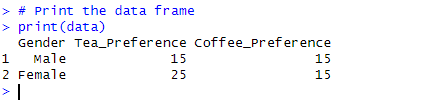

# Create a contingency table from the data
contingency_table <- matrix(
  c(data$Tea_Preference, data$Coffee_Preference),
  nrow = 2,
  dimnames = list(Gender = data$Gender, Preference = c("Tea", "Coffee"))
)

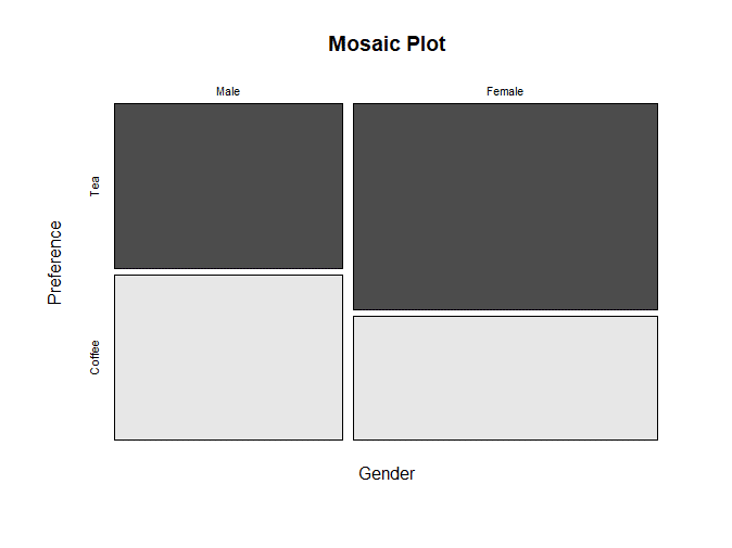
# Visualize using Mosaic Plot
mosaicplot(contingency_table, main = "Mosaic Plot", color = TRUE)

Expected frequencies

Calculating expected frequencies is an integral part of performing Fisher’s exact test. It serves several important purposes:

1. Comparison with Observed Frequencies: Fisher’s exact test determines the probability of observing the data in a contingency table (the observed frequencies) under the null hypothesis of independence. To calculate this probability, you need to compare the observed frequencies with what would be expected if the two categorical variables were independent (the expected frequencies). The test quantifies whether the observed deviations from expected frequencies are statistically significant.
2. Basis for the Test Statistic: The test statistic in Fisher’s exact test is based on the ratio of the observed frequencies to the expected frequencies. This ratio helps assess the strength of the association between the two categorical variables. A larger difference between the observed and expected frequencies will result in a more extreme test statistic.
3. Determination of Significance: Fisher’s exact test calculates the probability of observing data as extreme as the observed data under the null hypothesis. To do this, it considers all possible tables with the same marginal totals (row and column totals) as the observed table. The expected frequencies are used to calculate the probabilities of these alternative tables. If the observed table is significantly different from what is expected under the null hypothesis, it suggests a significant association between the variables.

To calculate the expected frequencies for a contingency table in the context of Fisher’s exact test, you can use the following formula:

Expected Frequency = (Row Total × Column Total) / Grand Total

# Calculate the row and column totals
row_totals <- rowSums(contingency_table)
col_totals <- colSums(contingency_table)

# Calculate the grand total
grand_total <- sum(contingency_table)

# Initialize a matrix for expected frequencies
expected_freq <- matrix(0, nrow = 2, ncol = 2)

# Calculate expected frequencies for each cell
for (i in 1:2) {
  for (j in 1:2) {
    expected_freq[i, j] <- (row_totals[i] * col_totals[j]) / grand_total
  }
}

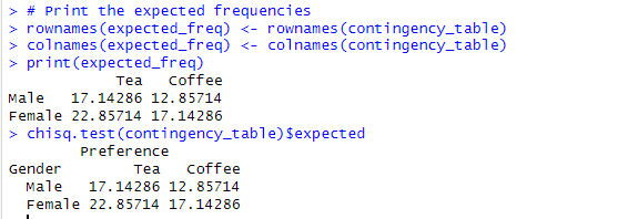
# Print the expected frequencies
rownames(expected_freq) <- rownames(contingency_table)
colnames(expected_freq) <- colnames(contingency_table)
print(expected_freq)

Alternatively, to obtain the expected frequencies, use the chisq.test() function in conjunction with $expected:

#Expected frequencies
chisq.test(contingency_table)$expected

Output:

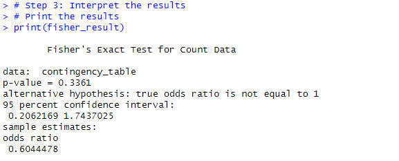
# Step 2: Perform Fisher's exact test
# We use the fisher.test() function to conduct the test

# Perform Fisher's exact test
fisher_result <- fisher.test(contingency_table)

# Step 3: Interpret the results
# Print the results
print(fisher_result)

# Extract the p-value from the result
p_value <- fisher_result$p.value

# Check if the association is statistically significant (using a 0.05 significance level)
if (p_value < 0.05) {
  cat("There is a significant association between Gender and Beverage Preference (p-value =", p_value, ")\n")
} else {
  cat("There is no significant association between Gender and Beverage Preference (p-value =", p_value, ")\n")
}

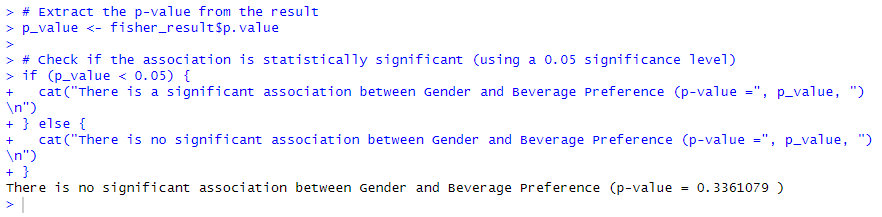
The code then extracts the p-value from the test result and checks if the association is statistically significant at the 0.05 significance level. The output will indicate whether there is a significant association between gender and beverage preference based on the p-value.

Additional Resources

• Hypothesis Testing in R
• How to conduct Sobel test in R