Introduction
The Exponentially Weighted Moving Average (EWMA) is a statistic for monitoring the process that averages the data in a way that gives less and less weight to the data as they are further removed in time. Like a cusum chart, an EWMA chart is an alternative to a Shewhart individuals or \overline{x} chart and provides quicker responses to shifts in the process mean than either an individuals or \overline{x} chart. This is because it incorporates information from all previously collected data.
The EWMA algorithm is an approach for forecasting values in a time series. The algorithm gives more weight to recent values in the time series, and less weight to older values.
EWMA also acts as a statistical tool that is used to smooth out data points in a time series. It does this by taking a weighted average of the data points, where the weights are exponentially decaying. This means that recent data points are given more weight than older data points. EWMA is often used to predict future values in a time series. This is because it can smooth out short-term fluctuations in the data and make the trend more visible.
Construction of EWMA Chart
To construct an EWMA chart, we assume we have K samples of size n ≥ 1 yielding K individual measurements X_1,…,X_k (if n = 1) or k sample means \overline{x}_1,…,\overline{x}_k , (if n > 1).
EWMA Formulas
Let Z_i be the value of the exponentially weighted moving average at the i^{th} sample. Then , for n = 1;
i=1;Z_1=\lambda X_1+\left(1-\lambda\right)Z_0;and for n >1;
i=1;Z_1=\lambda\overline{X}_1+\left(1-\lambda\right)Z_0;Similarly, for i =2;
i=2;Z_2=\lambda X_2+\left(1-\lambda\right)Z_1;and for n > 1;
i=2;Z_2=\lambda\overline{X}_2+\left(1-\lambda\right)Z_1;and so on.
It can be shown that for any \begin{array}{l}i\ \ge1\end{array} and n = 1
Z_i=\lambda\sum_{j=0}^{i-1}\left(1-\lambda\right)^jX_{i-j}+\left(1-\lambda\right)^iZ_0Similarly, it can be shown that for any i\ \ge1 and n >1
Z_i=\lambda\sum_{j=0}^{i-1}\left(1-\lambda\right)^j\overline{X}_{i-j}+\left(1-\lambda\right)^iZ_0Note that 0<\lambda\le1 is called the weighting constant and it controls the amount of influence that previous observations have on the current EWMA Z_i
Remarks
Values of \lambda near 1 put almost all weight on the current observation. That is the closer \lambda is to 1, the more the EWMA chart resembles a Shewhart chart. (In fact, if \lambda=1 , the EWMA chart is a Shewhart chart).
For values of \lambda near 0, a small weight is applied to almost all of the past observations, and the performance of the EWMA chart parallels that of a cusum chart.
If a target value \mu_0 is specified, then Z_0=\mu_0 . Otherwise, it is typical to use the average of some preliminary data. That is, Z_0=\overline{\overline{x}}
Variance of EWMA
The variance of Z_i for n = 1 is given by:
\sigma_{z_i}^2=var\left(Z_I\right)=Var\left(\lambda\sum_{j=0}^{i-1}\left(1-\lambda\right)^jX_{i-j}+\left(1-\lambda\right)^iZ_0\right)=\frac{\lambda}{2-\lambda}\left(1-\left(1-\lambda\right)^{2i}\right)\sigma^2The variance of Z_i for n\ \ge1 is given by:
\sigma_{z_i}^2=var\left(Z_i\right)=Var\left(\lambda\sum_{j=0}^{i-1}\left(1-\lambda\right)^j\overline{X}_{i-j}+\left(1-\lambda\right)^iZ_0\right)=\frac{\lambda}{2-\lambda}\left(1-\left(1-\lambda\right)^{2i}\right)\left(\frac{\sigma^2}{n}\right)EWMA Limits
The limits for n = 1 are given as:
UCL_i=\mu_0+L\sigma^2\sqrt{\frac{\lambda}{2-\lambda}\left(1-\left(1-\lambda\right)^{2i}\right)};i=1,…,Kand
LCL_i=\mu_0+L\sigma\sqrt{\frac{\lambda}{2-\lambda}\left(1-\left(1-\lambda\right)^{2i}\right)};i=1,…,Kand the Limits for n\ \ge1 are given as:
UCL_i=\mu_0+L\left(\frac{\sigma}{\sqrt{n}}\right)\sqrt{\frac{\lambda}{2-\lambda}\left(1-\left(1-\lambda\right)^{2i}\right)};i=1,..,and
LCL_i=\mu_0-L\left(\frac{\sigma}{\sqrt{n}}\right)\sqrt{\frac{\lambda}{2-\lambda}\left(1-\left(1-\lambda\right)^{2i}\right)};i=1,..,Note
- L is usually fixed at 3
- if \sigma is unknown, then use \hat{\sigma}=S where S is the sample standard deviation.
Example of how to compute EWMA in R

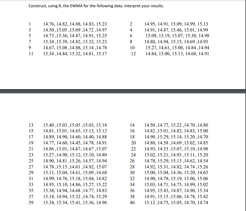
We are going to calculate the EWMA of the given data above. Note that there are five samples in each subgroup, making this multivariate data.

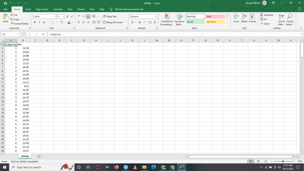
This is a preview of what your data entry should look like. You’ll need to do (40*5=200) entries. If thats a lot of work and you would like to follow along with this tutorial. Download the data set here.
#Loading the package qcc
library(qcc)

#Reading our dataset
charts.data <- read.csv("EWMA.csv")
charts.data
attach(charts.data)
This will load the R package qcc, which is a MUST in order for this code to work. Let me explain why it’s important to have the qcc installed.
The qcc package is used for quality control and statistical process control. It provides functions for creating control charts, calculating process capability indices, and analyzing process stability. The package also includes a variety of other quality control tools, such as sample size estimation and hypothesis testing.
Next we have;
#To view the first six data
head(charts.data)

#To view the last six datasets
tail(charts.data)
Output
#To view the first six data
head(charts.data)
subgroup   obs
1        1 14.76
2        1 14.82
3        1 14.88
4        1 14.83
5        1 15.23
6        2 14.95
>
#To view the last six datasets
tail(charts.data)
subgroup   obs
195       39 14.96
196       40 15.12
197       40 14.75
198       40 15.05
199       40 14.70
200       40 14.74
This is a preview of what your loaded data looks like. It’s standard practice to always check you are working with the correct data.
#creating a qcc object from the data
measurements <- qcc.groups(obs,subgroup)
head(measurements)
tail(measurements)

#Plotting EWMA
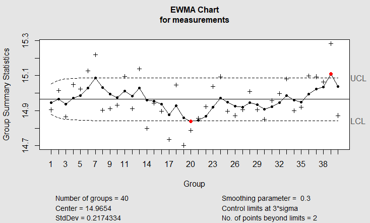
ewma(measurements, lambda = 0.3)
Output

