Definitions
A cumulative summation control chart is a type of control chart that is used to monitor changes in a process over time. This chart is used to detect small changes in the process that may not be detectable with other types of control charts. It is especially useful when monitoring processes that are difficult to control using traditional Shewhart control charts, such as those with large process variability or rare events.
The chart is constructed by plotting the cumulative sum of the deviations of each data point from the mean. If the process is in control, the plot will be a horizontal line. If the process is not in control, the plot will be a curved line.
The cusum control chart is based on the cumulative sum (cusum) of deviations from a target value. The target value can be the mean of a process distribution, or a specification limit. The cusum is calculated at each observation, and if it exceeds a pre-determined threshold, an out-of-control condition is indicated.
Just like the Xbar and R chart, the CUSUM chart is used to plot time series data, so the chart is meant to alert users to significant changes in process performance.
CUSUM charts do not plot raw data values, averages, ranges or standard deviations. Instead, plot points on a cusum chart are data values roughly representative of the cumulatively summed, subgroup to subgroup deviations from a specified target or production mean.
There are several advantages to using a cumulative sum (CUSUM) control chart over other types of control charts. One advantage is that CUSUM charts are more sensitive to small changes in the process mean than other control charts, such as Shewhart control charts. This means that CUSUM charts can be used to detect process changes more quickly.
Another advantage of CUSUM charts is that they can be used to monitor processes that are not in statistical control. This is because the CUSUM chart is based on the cumulative sum of deviations from the target value, rather than on the individual data points. This makes CUSUM charts more robust to changes in the process distribution.
CUSUM charts can be used to estimate the process mean, even when the process is not in statistical control. This is because the CUSUM chart is based on the cumulative sum of deviations from the target value, which is an estimate of the process mean.
Setting up a CUSUM Control Chart
When compared with traditional control charts, the tabulated CUSUM chart is unique, and certain parameters and statistics must be used in its creation.
- C_i^+=Max\left[0,\ x_i-\left(\mu_0+k\mu\right)+C_{i-1}^+\right] – The C_i^+ plot point is used exclusively for plotting the upper line on the tabular CUSUM chart. The upper line is used for identifying changes in the process above the stated target value, \mu_0
- C_i^-=Min\left[0,\ x_i-\left(\mu_0-k_l\right)-C_{i-1}^-\right] – The C_i^- plot point is used exclusively for plotting the lower line on the tabular CUSUM chart. The lower line is used for identifying changes in the process below the chosen target value, \mu_0
- \mu_0 – This is the process mean or target value e.g \overline{\overline{x}}
- M_sZ_u – The positive shift in process mean that the CUSUM chart meant to detect in standard deviation units. Typically between 0.5\sigma\ and\ 1.5\sigma
- M_sZ_l – The negative shift in process mean that the CUSUM chart is meant to detect in standard deviation units. Typically between 0.5\sigma\ and\ 1.5\sigma
- ku=\frac{M_sZ_u\cdot\hat{\sigma}_{LT}}{Z} – The upper reference value specified for plotted positive CUSUM line. Positive CUSUM values are accumulated only when the deviation from the target values exceeds specified K value. K value is half the magnitude of the mean shift value to detect.
- kl=\frac{M_sZ_l\cdot\hat{\sigma}_{LT}}{Z} – The lower reference value specified for plotted negative CUSUM line. Negative CUSUM values are accumulated only when the deviation from the targer value exceeds specified K value.
- h – The decision parameter. The factor of determining the decision interval, H. Generally h is defined as 5 also sometimes 4 is utilized.
- H=h\sigma – H is the decision interval which acts as the control limit.
Example of CUSUM Control Chart
| Sample | Diameter |
|---|---|
| 1 | 2, 6, 3, 8, 5 |
| 2 | 8, 8, 7, 7, 9 |
| 3 | 6, 2, 2, 4, 3 |
| 4 | 5, 6, 7, 6, 10 |
| 5 | 8, 2, 6, 5, 0 |
Construct the CUSUM chart and interpret the findings using R
solution
Before we start, we need to do data entry for the data above. Here is a screenshot of how your data should look like;

R code for CUSUM Control chart
library(qcc)
data <- read.csv("AA.csv",header = T)
head(data)
sample diameter
1      1        2
2      1        6
3      1        3
4      1        8
5      1        5
6      2        8

diameter <- qcc.groups(diameter,sample)
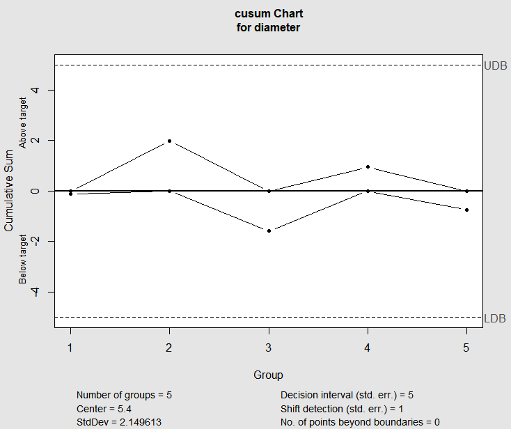
cusum.chart <- cusum(diameter, decision.interval=5,se.shift=1)
summary(cusum.chart)

Call:
  cusum(data = diameter, decision.interval = 5, se.shift = 1)

cusum chart for diameter

Summary of group statistics:
  Min. 1st Qu.  Median    Mean 3rd Qu.    Max.
4.8     5.0     5.4     5.4     5.8     6.0

Group sample size:  5
Number of groups:  5
Center of group statistics:  5.4
Standard deviation:  2.66552

Decision interval (std.err.): 5
Shift detection  (std. err.): 1
>
Output:

